Tips&Procedures
McNamara 20210119Tue (start) Tips and Procedures (also available as docx, PDF from GM)
* 20220104U: minor edits to web page (but not PDF).
George McNamara, Ross Fluorescence Imaging Center, G.I. Division, Dept of Medicine, School of Medicine, Johns Hopkins University. gmcnamara@jhmi.edu 305-764-2081, office ross Bldg S913 (service corridor).
URL: http://confocal.jhu.edu/mctips/tipsprocedures
* confocal microscope users may find of interest our 3/2021 Confocal Sweetest Spot web page http://confocal.jhu.edu/mctips/confocalsweetestspot
Purpose of this document: (i) provide tips on fluorescence microscopy in the context of our microscopes, (ii) provide brief procedures for our major instruments. We note this is “dense packed” with a lot of information and details; our goal is to put a lot of (hopefully) useful information in one place; we realize some of our users are brand new graduate students, postdocs transitioning from pure molecular biology/biochemistry to cells/tissues and microscopes, medical students or fellows doing lab rotations, lab technicians, new PIs, or even experienced PIs. All of you have made it this far in science and/or medicine (or engineering, etc), if you are motivated to learn and “do”, you will, and we can help.
I welcome feedback! Email is best, gmcnamara@jhmi.edu and happy to meet to discuss improvements, suggestions, etc (during covid-19 pandemic Zoom or Microsoft Teams may be best way to meet face to face). My apology that the tables currently do not display well on the web page – please contact me for Word doc (docx) or Acrobat (pdf) file.
While this is not clinical lab grade “standard operating procedures” (SOPs), we aim to provide good information, good advice and good practices for you. Intended audience are the researchers using or planning to use our image core for acquisition to help you do your experiment planning, sample preparation, imaging and analysis – usually graduate students, medical students, postdocs (with PhD and/or MD or equivalent), sometimes technicians, occasionally undergraduates, occasionally P.I.s. We advise and train at or close to the optical limits of our microscopes.
We are an image acquisition and advice core facility. Sample preparation (and controls) are your responsibility.
This document text is for our web site. Some Microsoft Word document formatting is deliberately simple, but may not transfer to our web site – you can get the Word document (or PDF) from George. Because of limitations of our web site, this document/page will avoid pictures. All our microscope PCs have Microsoft Word and Paint, you can always create your own documents (or work with George to do so). References are ‘in brief’. Image Core Manager George McNamara, has coauthored several articles and book chapters on light microscopy, immunofluorescence, and in situ hybridization (PubMed 32215866, 28696557, 27182204, 24052350, 26307258, 22475632, 16969821, 16969819, 16549508, 12533523) and Image Core Director Prof. Bin Wu is a leader in single molecule RNA imaging.
Responsibilities
We supply the microscopes, training, oversight, advice, lens paper, immersion oil, kimwipes, EtOH (clean your coverglass, spray down work areas, especially wrt covid-19 safety), ‘saran wrap’ (optional: cover keyboard, computer mouse, eyepieces, wrt covid-19 safety). Local data drive and Ethernet access to your JHU OneDrive (no USB drives allowed on any image core PC). We have some image analysis capability – most users use Fiji ImageJ in your lab on your own (we do not normally provide ImageJ training).
You supply and are responsible for:
Following our training and taking excellent care of our equipment while you are using it: don’t break our stuff! Take notes, ask questions (and remember answers); We note that Zoom enables recording sessions and we have microphones at most imaging systems, so easy to record (you are welcome to record your experiment sessions too). Zoom is
samples (coverglass recommended, either coverglass-slide or imaging dish)
understanding of your samples and controls (we recommend bringing a printout with details on each specimen, ex. Each pimary and secondary antibody and counterstain).
You promise to think through what you are doing to operate the microscopes safely, both instrument safety and biosafety for you, us, other users.
Saving to the fast local data drive on acquisition PC and before your session time ends upload to your JH OneDrive (the next user is allowed to start session on time). Reminder: no USB external drives allowed in our image core: we cannot risk computer viruses. Also, for same reason, do not “surf the Net” on our computers (looking online for your specific product information, such as Semrock Searchlight spectra web site, is ok).
No PHI: do not include any patient healthcare identification (PHI) information on your microscope slides, filenames, etc. As noted above, this is not a clinical lab. Your filenames and contents are visible to others.
New User Training
Most users will get two 2 hour training sessions on confocal microscopes, usually a single 2 hour session for other microscopes. All users should be computer literate with respect to Windows 10, JHU network (JH OneDrive), and your experimental details, prior to arranging training. Current microscope services are listed at http://confocal.jhu.edu/current-equipment and for full rates details see http://confocal.jhu.edu/facility-usage-fees
After the training sessions, each user is expected to be able to operate on your own – initially with oversight from Dr. McNamara, by limiting imaging sessions to JHU work hours, i.e. 9am-5pm Mon-Fri, and check in advance wrt vacation time.
Most users will get two 2 hour training sessions on either of our confocal microscopes they need to learn. FISHscope training usually takes 2 hours. Our other microscopes usually take 0.5 to 2 hours.
Standardizing training: we now (2/2021) normally start with our Eosin fluorescence slides, 20x/0.75 NA objective lens. Depending on user’s prior light microscopy experience and/or availability of their lab’s specimens, we may stay with our Eosin slide for longer or shorter time, before pivoting to user slides. We strongly encourage user’s to bring one or more bright, specific labeled, microscope slide(s) [or fixed specimen imaging dishes if that is standard lab methods) – for example tyramide signal amplification labeled slides are bright and stable.
Suggested reading (for browsing and reference, not ‘pre-med memorization’; both available on our file server [S:] and on data drive of most of our PCs – eBooks obtained through JHU electronic online library subscription):
Sanderson 2019 Light Microscopy.
Pawley 2006 Handbook of Confocal Microscopy, 3rd edition.
Additional microscopy eBooks on our file server, S:\Image Core Manuals\eBooks including:
Burry 2010 Immunocytochemistry: A practical guide for biomedical research.
Mondal Diaspro 2014 eBook - Fundamentals of Fluorescence Microscopy - Exploring Life with Light.
Paddock 2014 Confocal Microscopy (GM has chapter on low magnification confocal microscopy).
McNamara, G., Difilippantonio, M., Ried, T., & Bieber, F. R. (2017). Microscopy and image analysis. Current Protocols in Human Genetics, 94, 4.4.1–4.4.89. doi: 10.1002/cphg.42 (open access).
McTips
I have posted a large number of tips in four (annual) “McTips” documents
McTips 2017 https://works.bepress.com/gmcnamara/81
McTips 2018 https://works.bepress.com/gmcnamara/84
McTips 2019 https://works.bepress.com/gmcnamara/85
McTips 2020 https://works.bepress.com/gmcnamara/90
Along with my 2011 (started 1995)
Multi-Probe Microscopy https://works.bepress.com/gmcnamara/2 (our FISHscope with “RT” beamsplitter is a direct descendent of ideas from one section, see also http://confocal.jhu.edu/current-equipment/fishscope ).
Experiment design
Experiment design is your responsibility. We encourage you to talk/email with us for advice and recommendations on instrument choice, fluorophores to use (or avoid). The methods section of nearly all research papers are inadequate to perfectly reproduce a study (and should not need to do so, except for intent to replicate). Exactly matching settings would require using the same instrument with exactly the same settings (and sample prep): instrument performance changes over time and no two scientific instruments perform exactly the same (they can be tuned to close to a ‘lowest common denominator’, but this usually means they are not operating close to the theoretical optical limits of light). As noted above, we have published many articles and book chapters on light microscopy (see PubMed #s above).
Data
All data is owned by JHU and is the responsibility of the PI and user. By the end of each user session, the user should transfer their image data to their Microsoft OneDrive account (MyJHU à Cloud à “JH OneDrive”) and log out of both OneDrive and MyJHU (and never select a ‘store password’ option). The Image Core MAY – or not – back up user data. If we do have any PI/user data on the acquisition PC, file server, or backup, it will be available to the PI (and by implication, the user) or their dept/division; any outside requests should be sent to, and handled by, the PI. We strongly encourage PI/user to organize ALL their image data for each project and post it online at JHU’s https://craedl.org - Craedl, the Collaborative Research Administration Environment and Data Library (consider posting to Craedl for your electronic preprints, see Craedl policies). As noted above, no PHI – protected healthcare information – on specimens, filenames, or metadata.
Acknowledgements
Please acknowledge the image core for any instrument used. Some instruments were purchased with grant funds and the specific grant number should be in your manuscript (see instrument page at our confocal.jhu.edu web site). We welcome acknowledgement of image core staff contributions, when appropriate. We generally will not be co-authors on manuscripts, with exceptions involving scientific contributions (ex. Data interpretation and analysis).
Sample preparation
Specimen preparation is your responsibility. We provide some suggestions and some ‘anti-recommendations’.
Standard fluorescence microscopy uses a coverglass-slide. The imaging is done through the coverglass, usually #1.5 thickness (nominally 170 um). The higher the resolution you need, the more stringent that you use the correct coverglass thickness (the slide side is ‘almost irrelevant’ except for ease of handling to clean to avoid background fluorescence). You could measure each coverglass with a high resolution caliper, or by standing on edge and measuring with a microscope). In practice, you can buy 170um thick coverglasses, either standalone (coverglass-slide) or as imaging dishes (mattek.com, cellvis.com, for examples). More on imaging dishes at bottom (20220608W update).
First Two Specimens to image for EVERY Session: Positive and ‘critical negative’ controls
We strongly recommend your first two specimens be:
#1. “full positive” specimen, ex. All primary + ALL secondary antibodies + DAPI.
#2. “Critical negative” specimen, ex. NO primary + ALL secondary antibodies + DAPI.
The “NO primary” antibodies specimen(s) should have PBS or similar applied to them at the same time that your positive specimen(s) have primary antibody applied. Be sure to do all washes independently (not use a Coplin jar or similar where antibodies or other reagents could cross contaminate). Additional controls depend on you, what you are doing, what records you have for the same reagents previously (and when that was).
àRichard Burry 2010 Immunocytochemistry: A practical guide for biomedical research, Springer (eBook available through JHU online access; also on our file server), chp10, fig 10.3 and 10.4 show nicely that SEVEN washes after the primary antibody is better than <7 washes (see chp for details), note: he keeps the specimen submerged (wet) at all times, so each wash step may not dilute as much as some other authors.
Recommend: 170um thick coverglass (high precision version of #1.5) or 170um thick coverglass imaging dishes. You may find useful perusing the ibidi catalog/web site for potentially useful formats (ibidi products are often 180 um cyclic olefin polymer, which is ‘just about as good’ as 170 um coverglass).
Advanced ‘trick of the trade’: We note that a thinner coverglass can be useful to image deeper into your specimen. Standard #1.5 coverglass is ~170um, #0 coverglass is ~100 um, which would enable imaging an additional ~70 um into your specimen (useful distance depends on actual thickness of the coverglass [range 80-130 um], nominal working distance of the objective lens, refractive index of the mounting medium and immersion medium) (see http://www.microbehunter.com/cover-glass-thickness-and-resolution/ for table of all coverglass thicknesses). SiMPore manufactures special optically clear surfaces that can be much thinner (10 nm !!! see http://www.simpore.com/silicon-membranes note that these are small and fragile), some ibidi chamber slides incorporate these (one is a double perfusion chamber with pores in the special membrane; the imaging coverglass is standard ibidi ~180 um). We note that digital deconvolution (Leica SP8 HyVolution2, Leica Lightning or Thunder, Olympus cellSens GPU deconvolution) works best with ‘perfect refractive index matching’ of mounting medium and immersion medium.
Avoid: Lab-Tek chamber slides (4-well, 8-well), most other vendor’s chamber slides, either coverglass bottom or slide bottom. These flex and/or break easily: either is bad.
Tip: inspect each coverglass before you use it.
(i) when handling coverglasses, make sure that you only have a SINGLE coverglass. If two are stuck together, you will not be able to separate them and they will prevent high resolution imaging (and decrease quality of low resolution imaging). Hold the coverglass(es) up to the light and see if there are any interference patterns (“Newton’s rings”) or air gaps. Positive control: hold 2 coverglasses together. One reason we like imaging dishes is we have never (over decades) encountered a commercial imaging dish with two coverglasses stuck together.
(ii) coverglasses may not be absolutely clean out of the box (same applies to the slide). So: buy coverglass products that are as clean as possible AND consider cleaning them in your lab. There are a lot of protocols for cleaning class, some improve, some may make worse. There are also safety considerations (see Piranha solution in wikipedia). An example cleaning method is Faust 2018 JoVE DOI: doi:10.3791/56866 (Bo Faust, PhD, is now our local Olympus confocal microscope rep).
Imaging dishes: label the lid top near the edge AND label the side of each dish: if the lid falls off, you need to be able to identify the dish (especially if several lids fall off together). Do NOT let the specimen dry out EVER.
Reagents
è Old reagents may be bad (also: recent reagents may go bad or be delivered bad).
This is especially true after being in the refrigerator or lab shelf for several months during the Spring 2020 covid-19 lab closure. Age, contamination, many ways to fail. President Ronald Reagan’s quote, “Trust, but verify”, applies to your interaction with all your vendors (see “Santa Crap” below, for example) and your lab colleagues (ex. Leaving antibodies on their lab bench over a night or weekend and then putting them back in the refrigerator without admitting the mistake). You are responsible to yourself, your supervisor, your funding sources, and to Science, to do your work correctly, but you may not be able to rely on your colleagues or collaborators to treat common reagents well.
Some antibody vendors are unreliable, one, “Santa Crap” is both extremely unreliable AND unethical. With respect to the latter, S.C. was caught and fined by the U.S. USDA for hiding a herd of goats from the USDA inspectors (you can google the story to get the details on what bad things they were doing to the goats that led them to try to hide the herd).
Even antibodies from ‘good’ companies can go bad.
General Douglas Macarthur (1880-1964): “old soldiers never die, they just fade away”.
GM: “old antibodies die, please throw them away”.
Good vendors will provide recommendations on how to aliquot and store antibodies and other products. You/your lab should have a plan, and follow it, for storage and handling your reagents. I note that a vial of antibody left on a lab bench overnight or over weekend (instead of refrigerator) is likely bad (as is leaving it out all day).
$ antibodies vs imaging time: a typical primary antibody is $1/slide and fluorescent secondary is $1/coverglass (ex. $100 for 100 ug, use 1 ug per 20x20 mm coverglass or 20 mm diameter imaging area of imaging dish).
* Typical antibody experiments involve unlabeled primary antibodies, followed by washing, followed by secondary antibodies. We have observed many users skip critical controls. We urge users to start out each session with (in sequence, typically one field of view, avoid any air bubble):
All antibodies.
No primary antibodies, all secondary antibodies.
No antibodies (just DNA counterstain). …
***
20220504W note: Methods details matter! - Permeabilization anecdote
A user was unable to detect a transcription factor in the nucleus of their favorite cells (human intestinal epithelial cells monoloayers grown and differentiated on transwell monolayers from intestinal stem cell organoids aka enteroids). The user normally blocks (BSA etc) and permeabilizes (0.1% Saponin) simultaneously, washes, applies primary antibody. This failed to detect their transcription factor. They finally carefully re-read the methods section of the original paper, found the original authors used blocking step (BSA etc), and then 0.2% Saponin with the antibody(ies). Good thing the original authors provided "full details" in their Methods section.
More info:
Kimura 2019 JEM - Sox8 is essential for M cell maturation to accelerate IgA response at early stage after weaning in mice
page 12: After preincubation with 10% normal donkey serum for 1 h, the specimens were incubated with anti-Sox8 antibody, anti-Tnfaip2 antibody (Kimura et al., 2015), anti-GP2 antibody (MBL), anti–Spi-B antibody (R&D Systems), anti-RANK antibody (R&D Systems), or anti-RANKL antibody (BioLegend) in the presence of 0.2% saponin and 0.2% BSA in PBS overnight at 4°C, followed by incubation with appropriate secondary antibodies for 2 h at room temperature.
Local user modification(s): commercial Sox8 RAb at 1:100 in 0.2% saponin/0.2% BSA overnight at 4C, and I also added the 2o Abs in the same solution the next day for 1.5 hr at RT.
p.s. GM comment: I strongly discourage imprecise times in methods, especially "overnight". In a lab at Earth's equator, this is always 12 hours (not very friendly to a nominally 8 hour work day). At the North pole (everywhere north of the Arctic Circle), overnight may be as long as 6 months long, or need to wait 6 months to start the experiment. In between, varies by season. Istorngly recommend putting in exact time, ex. 16 hours, if done consistently, or a range, ex. 16-22 hour, if inconsistent (why? and does it matter? maybe you should pick a standard time interval and use that).
***
20220504W note: nice methods tip - EDC to crosslink smFISH probe(s) to RNA target -- facilitate long term storage:
Wu 2022 CellRepMeth - Robust and sensitive in situ RNA detection using Yn-situ. Cell Reports Methods 2, 100201 -- https://doi.org/10.1016/j.crmeth.2022.100201
p4: Previous studies had identified carbodiimide fixatives that effectively crosslink the phosphate group of the cellular RNA with amine groups from the proteins (Pena et al., 2009; Sylwestrak et al., 2016). We thus developed a protocol to irreversibly immobilize RNA molecules by crosslinking them to formaldehyde-fixed proteins using 1-ethyl-3-(3-dimethylaminopropyl) carbodiimide (EDC). In 6-month-old tissue stored at -80 C, we observed a dramatic improve
***
Fluorescent Dyes
Standard of care: Alexa Fluor dyes from ThermoFisher (which acquired the developer, Molecular Probes). In 2020, ThermoFisher launched “Alexa Fluor Plus” secondary antibodies and Alexa Fluor Plus Phalloidin (F-actin label), ~3x brighter than their standard (non Plus) reagents (same dye, different linker).
* see Multiplex web page for discussion about Alexa Fluor 610-X (Maillard 2020 ChemSci).
https://www.thermofisher.com/us/en/home/life-science/antibodies/secondary-antibodies/fluorescent-secondary-antibodies/alexa-fluor-plus-secondary-antibodies.html
https://www.thermofisher.com/search/results?query=alexa%20fluor%20plus%20phalloidn
Alexa Fluor dyes are often available from other vendors as well.
State of the art dyes (not intended to be comprehensive)
Janelia Fluor dyes (Tocris/biotechne) developed by Luke Lavis and lab at HHMI Janelia Research Campus – often highly photostable.
Mostly obsolete dyes (but can be inexpensive):
Cyanine dyes, aka CyDyes: Cy3, Cy3.5, Cy5, Cy5.5, Cy7. Can be cheap – especially bulk scale, see https://www.lumiprobe.com/p/cy3-nhs-ester
Some of the CyDyes ‘decompose’ when stored as oligonucleotides, M. Levitus 2020 Methods Appl. Fluoresc., doi.org/10.1088/2050-6120/ab7e10
page 14: For instance, the author has observed a steep decrease in the absorbance in the visible (but not in the UV) of buffered solutions of DNA labeled with the dye Cy5 stored for several months at −20 °C in the dark. While these storing conditions are typical for DNA samples, the Cy5 molecule seems to undergo an irreversible (and certainly unexpected) transformation.
More on ‘CyDeath’: see Gorka ... Schnermann 2018 Acc. Chem. Res. DOI: 10.1021/acs.accounts.8b00384
Amplification of Fluorescent Signals: Tyramide signal amplification (TSA) can increase signal by 100x AND you can start out by replacing the Diaminobenzidine (DAB) of standard immunohistochemistry (IHC) with horseradish peroxidase (HRP) and hydrogen peroxide (H2O2) with a fluorescent tyramide. An elegant paper by Belmont et al established diffusion radius of activated tyramide under different conditions (different reagent additives, ~50nm radius, which is sub-resolution on fluorescence microscopes; PMID: 30154186). Activated tyramide makes a covalent bond with tyrosine (occasionally histidine, rarely other amino acids), so is mostly resistant to washout (if the tyrosine is part of a protein fixed in the cell or tissue). A variant of TSA immunofluorescence is “APEX” live cell imaging, usually with biotin-tyramide and then mass spectrometry, amenable to biotin detection or use of fluorophore-tyramide (see APEX2 papers in PubMed and plasmids in addgene).
Quick Comparison of Fluorescent Signal for Different Immunofluorescence Approaches (many extinction coefficients and quantum yields are tabulated in McNamara 2017 CPHG https://currentprotocols.onlinelibrary.wiley.com/doi/full/10.1002/cphg.42 and in Fluorophores Table at http://www.geomcnamara.com/data [preliminary version of CPHG table]).
{my apology - table did not paste well from Word to web site editor}
Approach
Fluorophore
Degree of Labeling (DoL) wrt single antigen
Signal (DoL * fluorophore extinction coefficient [mM/cm-1] * quantum yield)
Direct label (Primary Ab)
Standard fluorophore – typical range
3
50 – 200
Direct label (Primary Ab)
Alexa Fluor 488 (modern classic ‘green’ dye)
3
200 (3 * 71 * 0.94)
Direct label (Primary Ab)
Brilliant Violet 421 (BV421)
1
1,500 (1 * 2,500,000 * 0.6)
Indirect (Primary + 2 secondary Abs)
Standard fluorophore – typical range
6
100-400
Indirect (Primary + 2 secondary Abs)
Alexa Fluor 488
6
400 (6 * 71 * 0.94)
Tyramide signal amplification
Alexa Fluor 488 - Tyramide
10 - 100
667 – 6,670 (10 to 100 * 71 * 0.94)
Note: in practice, ‘signal in practice’ depends on many variables beyond the simple photophysics of the ‘Signal’ calculation, including the quality of the antibodies and other reagents, other fluorophore details (photobleaching, aka photodestruction, pH of the mouting medium, ‘additives’ to the mounting medium, the microscope, the specimen, user skill in optimizing everything according to the needs of the experiment. Direct labels are more common in flow cytometry, where entire cell is one data point (about equivalent to a 1x objective lens on a microscope).
Fluorescent TSA vendors include:
Akoya Biosciences … Opal reagents (formerly PerkinElmer). Disadvantage: features Cy3 and Cy5 dyes (and complete kits only).
ThermoFisher (Molecular Probes): advantage: Alexa Fluor dyes (and lots of choices). The bottom of the SuperBoost TSA web page now lists ALL Alexa Fluor Tyramides as being available as stand alone reagents
this means you could substitute DAB with an AF###-Tyramide and continue using your other reagents (2ndAb-HRP, H2O2, etc); I note that fluorescent tyramide into a standard IHC autostainer could result in a very expensive run.
Tocris/biotechne: Disadvantage: features Cy3, Cy5 … may offer new fluorophores, such as Janelia Fluors.
Literature: “DIY” (Do-it-yourself) synthesis in labs has been published.
Commercial labs: “MultiOmyx” (aka MxIF) See https://neogenomics.com/sites/default/files/2020-11/MultiOmyx-Fact-Sheet.pdf NeoGenomics acquired the I.P. for “60plex” approach of Gerdes 2013 PNAS, McKinley 2017 JCI Insight, Herring … Lau 2017 Cell Systems, Bannerjee … 2018 JCI (originally developed by GE Global R&D); GM was involved the image analysis published in a ‘prototype 11plex’ of this approach, Santagata … Ince 2014 JCI.
à Special reagents:
I encourage use of Biocare Medical’s PeroxAbolish to “kill” HRP when multiplexing. I like this more than Akoya’s “heat/strip” or the Gerdes 2013 PNAS (GE Healthcare MultiOmyx) alkaline H2O2 or others.
Fitzgerald Industries sells POLY-HRP## a set of HRP polymer detection reagents (the $ HRP is 5x the number in the product name, ex. POLY-HRP40 has ~200 HRP per polymer molecule). Whether this or another 2ndAb-HRP polymer, the more HRP’s the more exposed tyrosine amino acids available for reaction with the activated tyramide radical.
“Next gen tyramides” (???) – Sato et al 2015, 2017, have found that N-methylated luminol-fluorophore + HRP + H2O2 works ~10x better than fluorescent tyramide. If generalizable and commercializable, this could be a game changer for “TSA”. Sato S 2015 ACS Chem Biol 10: 2633−2640, DOI: 10.1021/acschembio.5b00440; Sato S 2017 ChemBioChem 18: 475 – 478, DOI: 10.1002/cbic.201600649.
Fluorescent Proteins
Please replace EGFP etc with AausFP1 !!! CRISPR/Cas9 was published 8/2012 (8+ years ago), and Gibsdon cloning and other “tools” are available to upgrade.
èAausFP1: Lambert GG … Shaner NC 2020 Aequorea’s secrets revealed: New fluorescent proteins with unique properties for bioimaging and biosensing. PLoS Biol https://journals.plos.org/plosbiology/article?id=10.1371/journal.pbio.3000936
Many users still in 2020 use EGFP. EGFP was developed in 1996 and is obsolete (do you dive a 1996 vehicle?). You should strongly consider moving to AausFP1, which is ~5x brighter and more photostable, https://www.biorxiv.org/content/10.1101/677344v2 (should either put in monomeric A206K mutation or generate tandem dimer (“tdAausFP1”, will be ~10x brighter than one EGFP; wildtype AausFP1 is a dimer, so A206K monomerizing mutation or “td” should be used); amino acid sequence in figure in main text, DNA sequence in supplemental file – we recommend doing your own human codon & other expression optimization, such as www.jcat.de [we have had good success with Epoch life Sciences, http://epochlifescience.com , such as Donowitz lab mOrange2 fluorescent protein plasmid]. I also note that the classic EYFP is 1 aa difference from EGFP (T203 à T203Y), so I expect AausFP1(T203Y) will be yellow and bright (yellow: red-cshifted excitation ~20 nm from AausFP1; I also note EGFP and EYFP are S65T). See Dickson 1997 Nature (https://www.nature.com/articles/41048 ). I also note Bogdanov 2016 JACS (DOI: 10.1021/jacs.6b00092) Y145L improves photostability for EGFP (S65T Y145L) and EYFP (S65T Y145L T203Y) (their fig 8f). I have lots more suggestions on FPs, having followed the field closely science the 1994 Science paper (PMID 8303295) that won Martin Chalfie the Nobel Prize (unfortunately Doug Prasher was unable to share the award). In 2007 I published a book chapter, “a thousand proteins of light” (https://works.bepress.com/gmcnamara/86, https://works.bepress.com/gmcnamara/87 ), there are now a lot more FPs (see www.fpbase.org , interactive chart https://www.fpbase.org/chart works well with Y-axis = Brightness, X=axis = emission maximum), of which AausFP1 is brightest.
Confocal vs Widefield
Confocal is great. Widefield is great. Which to choose? Yes, each is useful.
Confocal: versatile settings (optimize or un-optimized), slightly better resolution possible (dxy = 0.51 * Lambda / NA for confocal; dxy = 0.61 * lambda / NA for widefield).
Widefield: not so versatile, resolution can only be obtained with objective lens à magnification optics à camera pixel size, are optimized. Image acquisition exposure is simultaneous for all pixels, for example, 1 second (1 million microseconds) for all 4 million pixels (FISHscope camera 2048x2048 pixels). Illumination is entire field of view (usually match the eyepiece field of view, which is somewhat larger than camera field of view).
Confocal light path: Maximum field of view and pixel size are under user’s control (often mis-control). Image acquisition exposure is sequential, by scanning each pixel sequentially (optionally with line averaging or “line accumulation” (add, sum), for example, setting confocal to 2048x2048 pixels, and using 10 microsecond total pixel dwell time (TPDT, ex. 2 usec * 5 line average on FV3000RS), total exposure time is ~4 seconds = ~4,000,000 microseconds (we normally scan unidirectional, with laser beam blanked ‘on the way back’, same speed as forward, so acquisition time is ~8 seconds). That is, confocal takes longer to acquire same field of view; each location (pixel) is exposure for much less time (10 usec) and at much higher intensity (all laser power into focused spot at resolution of the optics). Confocal is ~20% better resolution at standard pinhole size of 1.0 Airy units (which implies should use smaller pixel size, even more scanning time; confocal has adjustable resolution in that pinhole size <1.0 can be used, some examples: Jeff Reese (NIH) likes has his “confocal sweet spot” 0.6 to 0.7 Airy units ~8% to 12% better resolution; I suggest “confocal sweetest spot” of 0.666 Airy units, ~10% better resolution (more consistent setting than Jeff’s range); 0.5 airy units, ~15% better resolution; but also pinhole area [pi*r^2] is 0.25 so photon collection is 0.25, very few photons à very noise image); 0.2 airy unit ~20% better resolution but pinhole area is 0.04 so photon collection is 0.04, extremely few photons when imaging standard fluorophores (not a problem for reflection confocal microscopy; see Sivaguru 2019 https://pubmed.ncbi.nlm.nih.gov/31237354/ ).
Widefield light path: Maximum field of view and pixel size are fixed: Usually “magnification optics” is a 1x C-mount adapter; sometimes an “optovar” turret is purchased and installed in the microscope (ex: 1x, 1.25x, 1.6x, 2x), providing flexibility (but adds money, complexity, and precludes potentially more useful components in that part of the light path). For our FISHscope, we made the deliberate decision to not buy an optovar (saved money, un-versatile) and to buy a 1x C-mount (no glass). As a consequence, the specimen pixel size is dictated by the objective lens and the Hamamatsu ORCA-FLASH4.0LT pixel size of 6.5um, so for our 60x/1.4NA objective lens, pixel size is 108nm (that is: XY is 108x108nm) even though the theoretical resolution of a 1.4 NA lens is dxy = 0.61 * 500 nm / 1.4 = 214nm and therefore optimal pixel size would be dxy/~3.5 = 60nm (the ~3.5 being to account for Nyquist sampling in 2D). So: FISHscope is not “resolution limited” BUT bigger pixels (108x108nm) gets us more light per pixel than if we used ~60x60nm. The 108x108nm is still small enough that we can usefully spatially deconvolve the data, which usually results in a “very noticeable improvement” in contrast of single molecule RNA FISH puncta, many immunofluorescence signals, and DAPI (or Zombie NIR) DNA counterstain (note: contrast, not resolution; contrast and “brightness” are different things; details on these and signal-to-noise ratio, are “outside the scope” of this document).
Our Leica SP8 and Olympus FV3000RS are confocal laser scanning microscopes. “Laser scanning” refers to the use of the two scanning mirrors, usually mounted on galvanometers (“Galvos”) to scan a laser spot across the specimen, and then de-scan the collected fluorescence (photons) into the confocal pinhole and then the rest of the detection path (usually a set of beamsplitters and photomultiplier tubes (PMTs); in Leica SP8 two HyD hybrid photon counting detectors instead of PMTs). Conventional PMTs benefit from optimization of HV (high voltage; optimal is 500 mV on FV3000RS PMTs) and offset (usually adjusted so “no light” results in ~50 counts above zero for 12-bit = 4096 values); The Leica HyD’s are great because (i) higher quantum efficiency than PMTs, and (ii) photon counting mode is simple: the value is the number of photons, and (iii) Leica and Hamamatsu have optimized the hardware (no HV, offset or other settings for a user to mess up; I note Leica introduced POWER detectors in May 2020: even higher quantum efficiency, faster photon counting, FLIM capable … but requires new Leica STELLARIS 5 or 8: users are welcome to buy us one or more STELLARIS confocals).
Details: see Jim Pawley (editor) 2006 Handbook of Confocal Microscopy (we have the eBook PDF on our file server – or you can access directly through JHU library online access) and other reference books.
Confocal microscope hardware Tip(s) with respect to fluorescence
èFind the settings that get you the best data. Do not assume any default settings from the manufacturer OR any published settings in scientific papers (or protocols from your own lab) are optimal in any way. We teach using settings at the “optima XY” spatial resolution limit of the objective lens. See below for how these interact for resolution, brightness, scanning time (and money).
Confocals: Our main objective lenses are 20x/0.75NA dry and 60x/1.4NA oil (Leica SP8) or 40x/1.25Nam 100x/1.35NA silicone oil (Olympus FV3000RS). Our recommended pixel sizes (XY) and Z-step sizes are:
dxy = 0.51 * Lambda / NA … XY resolution for confocal microscope at 1.0 Airy unit, 500nm wavelength (Lambda).
Pixel size = dxy / 3.
Z = Pixel size * 3.
0.75 NA: 120x120 nm XY and 360 nm Z
1.40 NA: 50x50 nm XY and 150nm Z … Leica SP8
1.25 NA: 80x80nm XY and 240nm Z … Olympus FV3000RS
1.35 NA: 60x60nm XY and 180nm Z … Olympus FV3000RS
We encourage using GPU deconvolution on all Z-series (Leica/SVI HyVolution2 also works on single plane).
Confocal Critical settings AND they interact:
Total Pixel Dwell Time (TPDT).
Laser power
Spectral emission window[s]
Master beamsplitter (lasers in, fluorescence out) and emission path dichroic beamsplitters.
Amount of averaging or accumulation (photon count sum).
Pixel size, which depends on zoom and image format:
Zoom
Image format (ex. 512x512, 1024x1024, … 8192x8192 pixels … other values available).
That is, zoom 2X & 1024x1024 pixels and zoom 1X & 2048x2048 pixels results in same pixel size (on Leica SP8, will be different TPDT).
Z-step size. This is typically 3X bigger value than the optimal XY pixel size. Tip: always do Z-series moving “up against gravity”, because the Z-drive motor behaves better going up.
Working distance: is determined by the objective lens (high NA will have small working distance). Your coverglass thickness + specimen thickness determines how far you can image into your specimen. Microscope objective lenses are all designed to image “just past” the coverglass, ex. 4 um thick H&E tissue section. All objective lenses can image this, if you used the correct coverglass (and if only one coverglass: sometimes 2 get stuck together, so best practice is to inspect each to make sure only one [yes, doable]). As described elsewhere in this doc, standard is #1.5 coverglass (170 um), but you may sometimes (rarely? Often?) benefit from a thinner coverglass (ex. #0 is ~100 um, gaining an extra 70 um working distance).
Optional: spatial deconvolution. We have GPU deconvolution for each confocal (SP8 HyVolution2 on the SP8 PC; FV3000RS and FISHscope uses cellSens on the FISHscope PC, 10 Gbe Ethernet connection with our file server [hopefully by end of 2020 also 10 Gbe for JH OneDrive).
Optional: spectral (multichannel) unmixing. Our Leica and Olympus software do not have ‘great’ (or even good) spectral unmixers (we are an image acquisition core, not so much image processing or analysis, so you are on your own: Fiji ImageJ has several plugins that try to do this, good luck validating on your own data that any work). If you are, or know (and have money to pay for) software development, we have references and suggestions. Especially Adam Hoppe’s 3DFSR – PMID 18339754 (2008), 23762252 (2013) – reporting 10x improvement in signal to noise ratio (SNR) by performing joint spatial deconvolution and spectral unmixing (“JSDSUN”; a simple way to think about 10x SNR is: would you like to get paid 10x more money? We have Hoppe’s Matlab code: need someone to modernize it and enable running on GPU).
Unidirectional vs Bidirection scanning: Note: We always use and train with unidirectional scanning because bidirectional (i) risks mis-alignment forward and back (even if subtle, not worth risking it our opinion), and (ii) photobleaching rate may differ (faster on ends; if you know or think you need bidirectional, great: you can figure out how to turn it on (please turn off before next user) or I can show you. If you use bi-directional and later discover mis-alignment, too bad: you get what you pay for, we charge you the same if you acquire nice or poor images, but please blame yourself not us for your settings.
Many of these settings interact (and interact differently on SP8 vs FV3000Rs vs other confocals). In principle, you should report (in your lab notebook, electronic lab notebook, lab meeting PwoerPoint presentation notes, manuscript, publication, online data repository) ALL your settings (most are in the metadata in the native image file format) and important values like TPDT that may not be explicit in the metadata. Simple approach: acquire a screen shot (alt-PtrScrn keystroke) to copy to Windows clipboard, paste into Paint (Paint app, aka pbrush), and then save to your current data folder (and upload to your JH OneDrive).
We recommend not changing too many settings during a session – especially since they may interact.
“Faster is better”: fast scan speed, with averaging (FV3000RS) or line accumulation (SP8 HyD “counting” mode), is better.
Slow is BAD for fluorophores: (i) photobleaching, (ii) phototoxicity (if live cell). These are nonlinear effects, that is, 2x more photons (slow scan speed = long pixel dwell time, and/or higher laser power) results in >2x photodamage. Easiest way to demonstrate this is to zoom 10x (to limit field of view) and scan the way we recommend (600Hz on SP8 [10 line accumulation, photon count mode HyD], 2 usec * 10 line average on FV3000RS) and then test at 1/10th speed (60 Hz on SP8 [no accumulation] or 20 usec [no averaging] on FV3000RS). Post-acquisition can scan (fast settings) at say 5x zoom to see effects of photobleaching. Test on a not-valuable field of view.
Scan speed on our point scanning confocal microscopes:
Default Leica SP8 scan speed is 400 Hz (400 lines per second). I always start with 600 Hz. 16-bit data mode (not 8-bit or 12-bit), 10 line accumulation (adjust to fewer or more depending on data quality, 1% laser power, HyD detector(s) in photon counting mode (that is, I train all SP8 users to use 600Hz or higher speed, 600/400 = 1.5x sped, then use line accumulation [sum] to ADD photons, not average (since averaging 0's lowers the data values) … and started doing this with the SP5’s I managed in Miami starting in 2007 – Jonathan Boyd, at the time, Leica applications scientist, demonstrated “faster is better” [same total pixel dwell time]) because 600 Hz works at Leica’s “0.75x” zoom (their “philosophy” is their standard of care is 1x zoom, but they enable zooming down as far as 0.75x so users can choose to get a bigger field of view).
Our Olympus FV3000RS can operate in “galvano” (galvanometer, aka “galvo”) or resonant (RS) scanner modes. Galvo mode is 2 usec (microseconds). I often use 5 line averaging, so 10 usec TPDT, in galvo mode. Total scan time then depends on image format (ex. 512x512 or 4096 pixels) and number of Z-planes. The RS mode is 16x faster and limited to 512x512 pixels. Maximum 16 averaging (usually 16 line averaging), which is ~1 second per image (a user could “do’ more averaging later by acquiring time series or Z-series and then averaging in MetaMorph, Fiji ImageJ, etc).
|
20220104U (almost all text from a 20200204Mon draft appnote): more narrative on leica SP8 scan speed ... Leica SP8 confocal microscope – Faster scan speed for less photobleaching The main goal of this note is that fast(er) scanning speed + appropriate number of HyD line accumulations produces better data for the same “total pixel dwell time” (tPDT) than Leica defaults, mostly by decreasing photobleaching. I also compare other default settings vs my preferred settings. The Leica LAS X software TCS mode defaults to 400 Hz and XXX * XXX pixels, resulting in a pixel dwell time of 0.XX usec (XXX nsec). The interface default for the HyD’s are “standard” (if you do not have the definition memorized, you should read the Leica manual for what this means) and XXX averaging. I never use the Leica TCS defaults. {tip: sometimes LAS X reports incorrect numbers - when in doubt, calculate for yourself ... remember that with Unidirectional scans, the X-scanner flyback is dark time, so 1 second acquisition time is ~500 ms laser on time). I use: 600 Hz (or faster), HyD photon counting, 10 line accumulation (may increase or decrease depending on resulting data and ‘time is money’ constraints). optimal X * Y pixels for the resolution of the objective lens (ex. 120 nm for 0.75NA objective lens, 50 nm for 1.4 NA objective lens, subject to ‘time is money’ constraints; XY confocal resolution = 0.51 * lambda / NA; simplified example: 0.5 * 500 nm / 1.4 = 178nm, my preferred pixel size with deconvolution is then 178 / 3.5 = 51nm; see also SVI.nl Nyquist calculator recommendation). I could show exemplary data, but instead recommend this test for you to perform on your specimen (on nearby, non-overlapping, fields of view you do not need): At zoom 1 and 600 Hz, acquire an uniform area (“pre-test series”). p.s. Our Leica SP8 has SVI.nl Huygens software and so use LAS’s HyVolution2 interface. This adds a “Fast Live” button, which has advantages over TCS Live button: (i) further away from the “Autofocus” button to decrease risk of damaging the microscope and/or specimen, (ii) fast, consistent setting (512x512 pixels, no line accumulation). Same tPDT, big difference in photbleaching.
Acknowledgment: Jonathan Boyd, PhD, when he was a Leica employee and I managed Leica SP5’s with tandem galvo and resonant scanners showed me the performance with galvo 80 Hz (no accumulation), 800 Hz * 10 accumulation, and RS mode 8000 Hz * 100 accumulations. The 80 Hz setting caused much more photobleaching (post scan dark square when reviewing the specimen by eye or zooming down in software). Note: you can set scanning speed to even slower than 80 Hz. Do it yourself (DIY): "Seeing is believing!" --> "Doing to believe". *** Additional tip: you can usually induce photobleaching by zooming into a small area, such as middle of one cell nucleus, while leaving other settigns constant. For example, if you increase zoom by 10x, then the area being scanned decreases by 100x, and the density of light into that area increases 100x. If you also increase laser power, from say 1% to 10%, optionally 10% to 100%, this will increase photobleaching. Leica LAS X has a time series dialog box (xyzt mode) if you want to capture the photobleaching data (HyVolution2 Fast Live button is fine to demonstrate to yourself the effect). I do note that the HyD detectors have a limited dynamic range (~400 photon counts per pixel [no line accumulation or averaging] and if you exceed the maximum for more than a few pixels, a safety interlock will trigger, and data will be black (zero) until you stop scanning. |
Reflection Confocal Microscopy (RCM)
àWe are big fans of reflection confocal microscopy. We usually don’t train new users on it, since very few are aware of it and few absolutely need it. Among the uses:
Consistent focus selection, i.e. set Z-start to coverglass-cell interface (first image plane would be half in glass, half at cell bottom). The more consistent your methods, the more consistent your data may be. A published example is Jiang … McNamara … Lossos 2010 Blood (PMID: 20844236; https://pubmed.ncbi.nlm.nih.gov/20844236/#&gid=article-figures&pid=figure-2-uid-1 also illustrates HeLa tetrads: 40 hours after plating HeLa cells at low density, get granddaughters whose 4-cell colony fits nicely in confocal 1.4NA objective lens field of view; paper also illustrates do not need to acquire entire Z-series: we acquired 0, 2.0, 4.0 um).
Interference reflection contrast microscopy (IRM) aka Reflection interference contrast microscopy (RICM) of the cell-substratum (coverglass) interface. Focal adhesion sites (ex. Fibronectin : integrin binding sites) are “zero nanometers” from the surface, so exhibit strong destructive interference, resulting in black pixels, at every wavelength (ex. 405, 488, 552, 638nm). Close contacts (underside of cell plasma membrane NOT in contact with coverglass) results in interference such that intensity (black to white) depends on distance, refractive index of everything (glass, culture media, plasma membrane, cytoplasm) and wavelength. Upshot is 2 or more wavelengths can be acquired and image computations performed to get absolute distance (“DW-RICM”, E. Sackmann; typically calibrate/verify using microsphere of known dimensions … I note triple wavelengths would resolve some ambiguities).
Reflections (aka scatter, backscatter) of “features” inside cells (also applies to fresh and fixed tissues).
Find the “top” of the cell(s) and/or microscope slide surface. “Top” is the far side of the cells, away from the objective lens – coverglass – cells. Enables consistent focusing and setting Z-top (Z-end: always go up against gravity). I note that you may want to start and end Z-series further than the coverglass-cells and top-of-cells: up to you (if doing deconvolution, at least 5 planes outside the cell should be included, or see deconvolution software manufacturer instructions for optimal # planes above and below).
Coverglass flatness topography and cleansliness: (i) any tilt, aka not perfectly perpendicular, to image plane [happens all the time, mostly due to how users mount coverglass on slide, or stick a label near one end of a slide], (ii) topography is how flat (unflat) your coverglass surface is (and paying more money may not get you more uniform thickness; whether topography matters for your experiment depends on whether your cells ‘get their groove on’), (iii) ideally coverglass should be clean (since unclean is likely to also be unreproducible). You may want to clean your coverglasses yourself (but ask: how reproducible is your process?). O2 plasma cleaner (several thousand dollars), Piranha solution (nasty to handle), many other methods, have been published. Our local Olympus confocal sales rep, Bo Faust, PhD, published (JoVE 2018) a nice method, doi:10.3791/56866
RCM see also
https://works.bepress.com/gmcnamara/72/ Light Microscopy Reflection Focusing Cells and Coverglass
https://works.bepress.com/gmcnamara/10/ McNamara 2012 Leica SP5 inverted IRM - HeLa cell images
Confocal settings interact: resolution, brightness (photon counts: TPDT), scan time (money) & more:
I will use our Leica SP8’s 20x/0.75 and 63x/1.4NA objective lens to explain how the settings interact. The SP8 scanner can zoom down to 0.75X zoom (or any zoom from that to 48X). If I zoom the 20x by 3X = 60x total magnification, I can match this by using the 63x with 0.95X zoom (really 0.95238, but in practice sub-nanometer differences not going to matter). I note here that we did not buy a 100x/1.4NA objective lens because we can zoom either the 20x or the 63x lens to 100x total magnification or any other total zoom that makes sense for your experiment (120x, 150x, 200x, 666x, max 960x for the 20x lens, 3024x for the 63x lens, either of which results in “silly small” pixel size). I note that the two objective lenses have different working distances (Z-focus range), and higher NA lenses usually perform badly at the far end of their Z-range (further from the coverglass) and/or if there is refractive index mismatch (especially if live cells or thick tissue, which usually cannot be perfectly refractive index matched). The working distance might be “extended’ by using a #0 coverglass (~100 um) or #1 coverglass (~130 um) instead of the standard #1.5 coverglass (~170 um), if the refractive index of the mounting medium (specimen side) is matched to that of the coverglass (~1.518 R.I. of glass): that is, could get an extra ~70 um working distance with #0 coverglass; I also note that http://www.simpore.com/custom (SiMPore Inc - Precision Membrane Technologies), offers special (though small) “membranes” of: Si 5 to 75nm, SiO2 20 to 4000 nm (4um), SixNy 5 to 2000 nm (2 um; silicon Nitride) (SiO2 = silicon dioxide is a type of glass, re: fiber optics).
Resolution (confocal): dxy = 0.5 * NA / wavelength (I will simplify slightly from the standard confocal 0.51 to easier to remember 0.50; reminder: widefield uses 0.61, which we simplify to 0.5, so confocal at 1.0 Airy unit is 20% better resolution than widefield, if pixel sizes are optimized and fluorescence is bright enough to get useful data from positive specimens [empty areas and negative controls typically close to zero photons]).
Brightness proportional (“B”) to NA^4 / Magnification^2 (NA to the fourth power divided by mag squared). Note: “proportional”.
So at the same total magnification of 60x, Brightness is simply proportional to NA^4. Since in this scenario, we are zooming to 60x for each, then
“B” 0.75: 0.75^4 = 0.316
“B” 1.4NA: 1.40^4 = 3.84
So: 1.4NA is 3.84 / 0.316 = 12 times brighter than 0.75 NA (in principle), for same pixel size (also assumes the fluorescence is localized within the resolution limited spot; hard to really tell because usually vastly different laser power at pixel [spot size] and total pixel dwell time, and detector quantum efficiency).
Procedures [stub]
Confocal microscope hardware [stub]
|
20211021H update - free software (note: "you get what you pay for") Fiji ImageJ and CellProfiler 4 Fiji ImageJ by default does not have the Bio-Formats plugin loaded. This is needed to open images in many of the file formats we use (Leica .LIF container files; Olympus VSI ... Fiji / Bio-Formats has problems with OIR files). To add Bio-Formats go to: Help ... Update (2nd menu item from bottom) ... Manage update sites ... "check on" Bio-Formats (list is alphabetical) ... Close (the Manage update sites indow) ... Apply changes ... then step back out of dialog boxes/windows, and restart Fiji ImageJ. Late 2021 - 3 useful reviews on Fiji ImageJ and/or Cell Profiler New Extensibility and Scripting Tools in the ImageJ Ecosystem. ImageJ and CellProfiler: Complements in Open-Source Bioimage Analysis. CellProfiler 4: improvements in speed, utility and usability. Stirling DR, Swain-Bowden MJ, Lucas AM, Carpenter AE, Cimini BA, Goodman A. BMC Bioinformatics. 2021 Sep 10;22(1):433. doi: 10.1186/s12859-021-04344-9. PMID: 34507520 Free PMC article. ** 20220801M update - see also napari.
|
</
|
20220104U: Antigen retrieval quick summary from Dunkenberger and Del Valle 2002 MMB 2422 (ref and URL below). *and see next row. In 1991, Shi et al. {Clive R. Taylor is best known pathologist from this group} described AR involving the submersion of FFPE tissues in boiling water, a process now known as heat-inducedepitope retrieval, or HIER [6]. HIER is generally superior in performance to PIER {proteinase induced epitope retrieval}, with the exception of epitopes that may be damaged during the heating process and thus on which HIER would be ineffective [7]. For optimal results, heating should be as even as possible, with at least 15–20 min of a constant boil recommended for HIER. Lower temperatures may also be used with extended incubation times [8]. Several different buffers may be used for HIER; citrate buffer at pH 6.0, EDTA buffer at pH 8.0, and Tris-EDTA buffer at pH 9.0 are most commonly employed. Buffer pH can have a dramatic effect on HIER efficacy and experiments should be performed to determine the optimal pH for AR of any specific epitope [9, 10]. Experiments have shown both citrate and EDTA buffers to be effective for HIER [7, 11]; however, Antigen Retrieval and Signal Amplification. Immunohistochemistry (IHC) offers a valuable method for determining the spatial distribution of proteins in cells and tissues. Fixation of tissues prior IHC enables their long-term stability and preserves tissue morphology; however, downstream analysis of protein localization within fixed samples can be complicated by cross-links formed between proteins during formalin fixation which mask target epitopes. Antigen Retrieval (AR) is a process introduced to reverse such cross-links, improving the sensitivity of antibody-based protein detection, and can be performed using protease- or heat-based approaches. Even following AR, low abundance target proteins may require additional amplification for sensitive visualization. The development of amplification approaches such as the use of biotinylated secondary antibodies with avidin-biotin complex and tyramide signal amplification greatly improve the sensitivity of IHC, enabling a wider range of epitopes to be detected when coupled with AR. Keywords: Antigen retrieval; Enzymatic; Heat-induced epitope retrieval; Proteases; Signal amplification.
|
|
|
More Antigen retrieval 20220425M: More Antigen retrieval - Bogen and colleagues have published a series of papers -- a few of many are listed below -- on antigen retrieval, including a model "masked antigen" with a defined chemically masked lysine that does not bind standard antibody, and can be chemically unmasked to enable antibody binding. This "lysine" vs "lysine-formaldehyde adduct" behavior could have been predicted from a pair of antibodes one binding "phospho-epitope" and the other the same peptide unphosphorylated. As might be expected, linear epitopes that do not have a lysine "in or near" the peptide epitope do not need (or benefit from) antigen retrieval. The papers also mention some antibodies bind to "conformational epitopes" with discontinuous amino acids (ex. 8 amino acids, with four on each of two different parts of protein molecule ... or occasionally on a heterodimer). PubMed search (only some hits on 20220425M shown): Quantitative comparison of PD-L1 IHC assays against NIST standard reference material 1934. Development and Validation of Measurement Traceability for In Situ Immunoassays. Quantitative Assessment of Immunohistochemistry Laboratory Performance by Measuring Analytic Response Curves and Limits of Detection. Molecular mechanisms of antigen retrieval: antigen retrieval reverses steric interference caused by formalin-induced cross-links. Experimental validation of peptide immunohistochemistry controls. ** Back to antigen retrieval big picture - there are only a few antigen retrival protocols and antibody vendors should state in their data sheet and product web page which one(s) to use -- and equally which to avoid. The usual protocols are: * pH 6.0 citrate buffer ... at "high temperature" * pH 10 buffer (not sure what chemical composition required] ... at "high temperature". --> the "high temperature" might be 60 C, 95 C, or other -- see the antibody protocol. Chemical stripping - optional for simple experiments, may be essential forsequential multiplex -- good starting point is ron Germain's multiplex papers -- see http://confocal.jhu.edu/mctips/multiplex -- Ron likes LiBH4 instead of NaBH4 -- please take the time to understand and follow safety rules for any BH4 Borohydride (chemical hood always, avoid water getting into bottle, follow instructions for mixing BH4 into other solutions).
|
|
&n
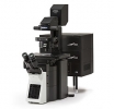
. Olympus FV3000RS Confocal MicroscopeOlympus FV3000RS Confocal Microscope Please acknowledge NIH shared instrumentation grant 1S10OD025244-01 (Prof. Brian... Read More
ACCM_IncuCyte_S3ACCM Incucyte S3 Live-Cell Imaging and Analysis System Live cell imaging system inside 37 C incubator - short to long term... Read More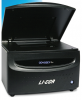
Li-Cor Odyssey CLxLi-Cor Odyssey CLx fluorescence scanner. This instrument is hosted by Prof. Donowitz lab and use is intended for G.I. Center... Read More
Zeiss Axio Observer.A1 Inverted Microscope (S972) Use iLabZeiss Axio Observer.A1 Inverted Microscope in Ross S972 has an Olympus DP80 RGB color + monochrome camera, capable of both RGB... Read More
. FISHscopeFISHscope Main application: single molecule RNA fluorescence in situ hybridization (smFISH). FISHscope Quick Tips web page... Read More |